


It’s been nearly two decades since the release of Google Sheets, and even all these years later, it’s still the go-to tool for creating charts and graphs.
But that doesn’t make it the most intuitive platform. And frustrating as it may be, it won't take long to learn the ropes.
This guide explains how to make a graph in Google Sheets, plus provides examples of charts and graphs so you can pick the right visualization for your needs. It also explains when you might need more than Google Sheets (like a professional-grade visualization tool for making TV dashboards).
Step-by-step: how to make a chart in Google Sheets
Here’s how to make a graph on Google Sheets in four steps:
- Copy/paste numerical data into your spreadsheet
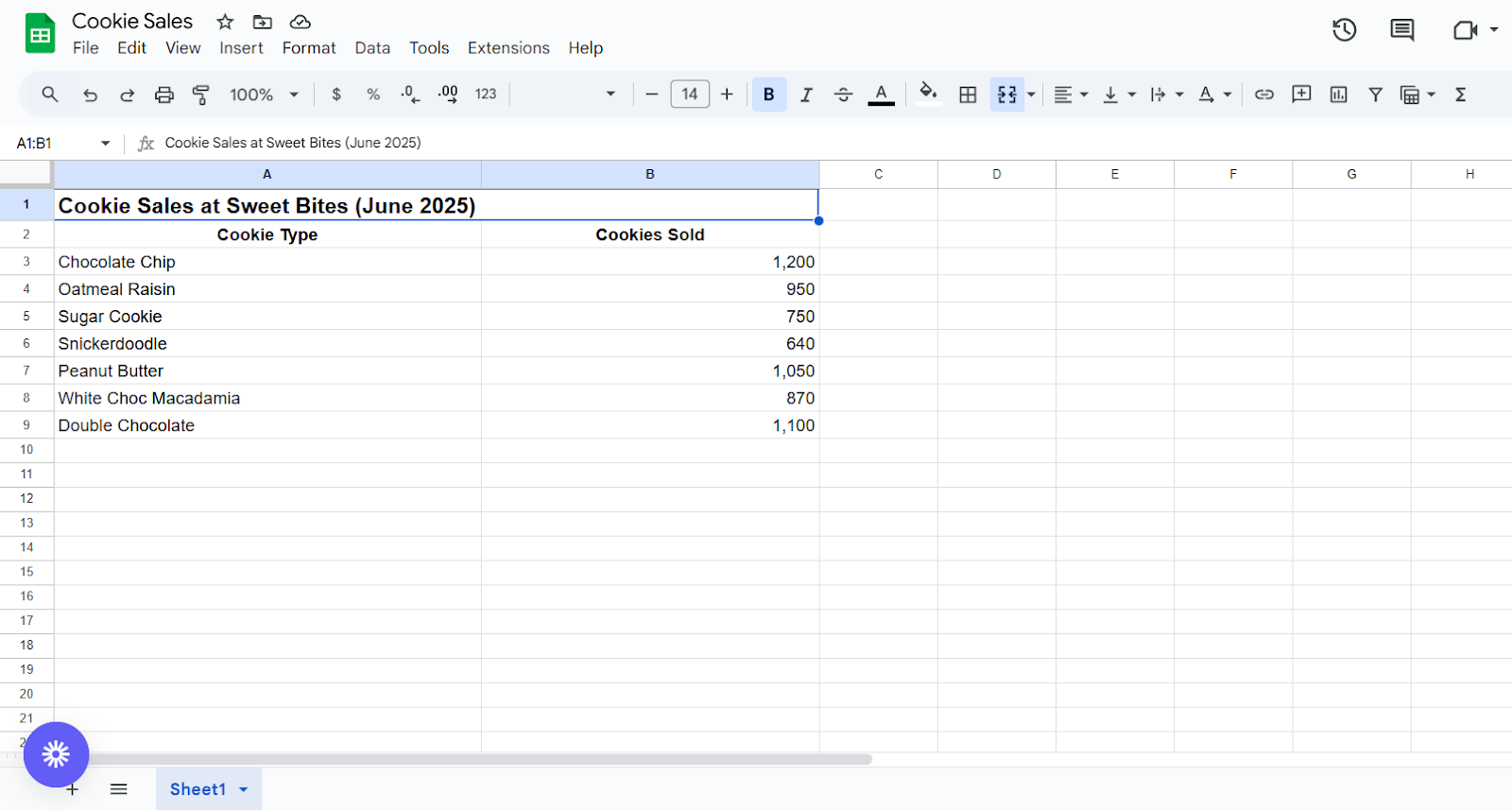
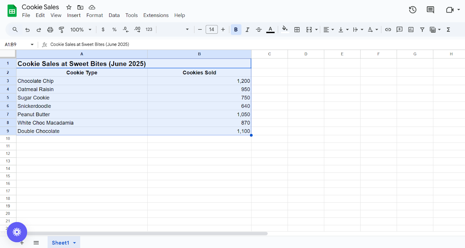
- Highlight the specific data set you wish to visualize. You can either use the keyboard arrows to select the entire data range (including headers), or click and drag your mouse over the selection.
- Click Insert → Chart.
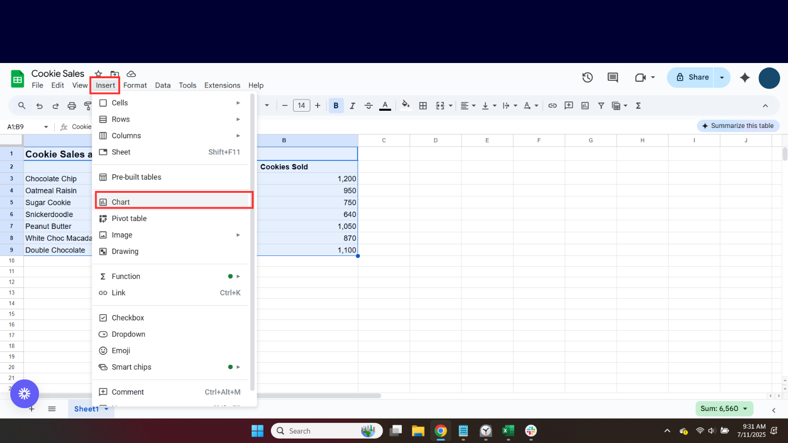
Google Sheets will automatically create a default chart based on your data.
- Next, select the chart type you wish to create, like bar chart, pie chart, line chart, etc. You can then customize the chart using the chart customization tab (think labels, colors, gridlines, axes, and legends). We’ll cover more about this later.
And that’s it! You’re done.
We explain how to change chart styles, format data points, and add axis titles later in the guide.
First: What kinds of graph types can you make in Google Sheets?
There are (technically) eight types of graphs, charts, and visual representations available in Google Sheets:
Pie chart: Best for depicting parts of a whole

A pie chart visualizes a set amount of data based on its percentage of a whole. In this sample data, you’ll notice that more chocolate chip cookies were sold than any other cookie, based on the total number of sales in a month.
Pie charts are best for looking at “part-to-whole” comparisons, but not necessarily direct comparisons like with bar charts.
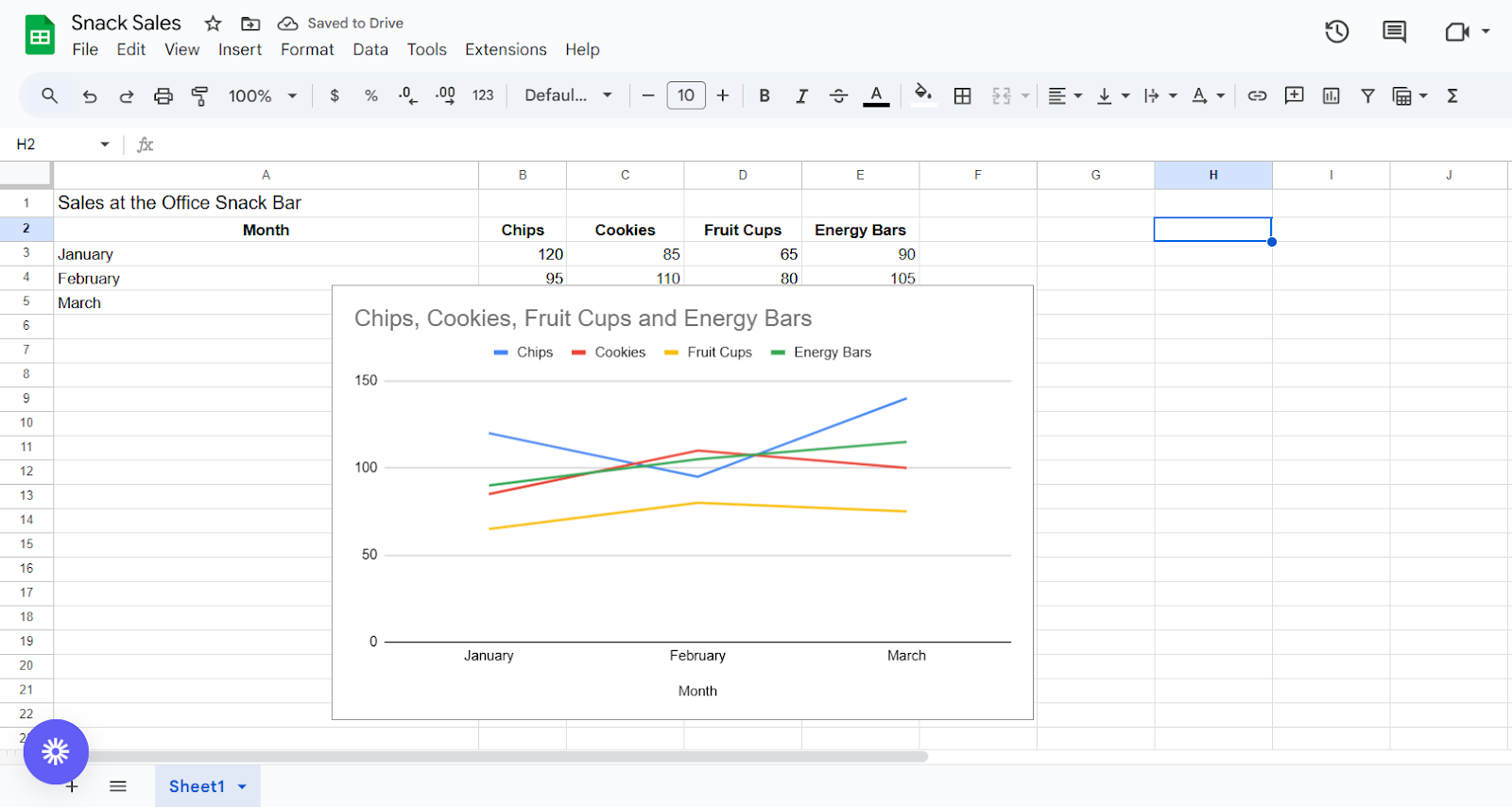
Line chart: Best for tracking trends

Line charts show trends over time by connecting data points with one (or more) continuous lines. They’re best for showing patterns, trends, or changes over time, especially if you want to highlight movement or progression.
Just keep in mind that line charts might be harder to interpret and sometimes confusing depending on the audience. They also don’t necessarily show all parts of the whole, so you might need to pair it with your raw dataset or another chart.
Bar chart: Best for simple comparisons

The quintessential bar chart is one of Google Sheet’s most popular options. It uses rectangular bars to compare different categories side by side (like if we wanted to compare popular beaches, for example).
Bar charts are ideal for making quick visual comparisons between groups, but they’re far more effective if exact numbers matter, or the differences between categories are particularly significant.
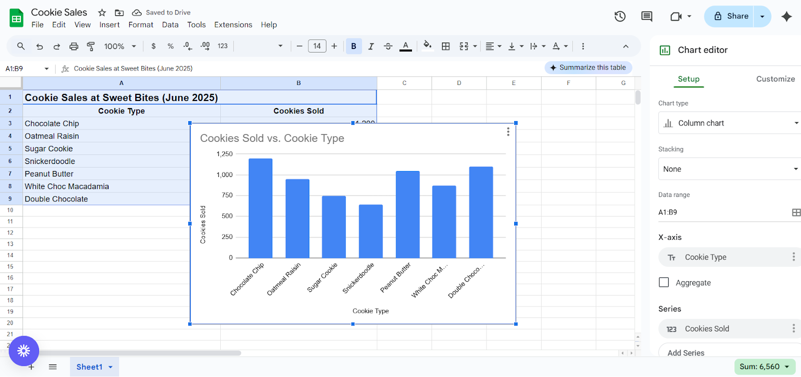
Column chart: Best for data changes over time

A column chart is basically a bar chart turned sideways — it uses horizontal bars to compare values across categories. For example, you might use a column chart to compare average rainfall by month, or look at the average amount of bubble wrap popped per department. 😉
Column charts are especially useful when you have fewer categories and want to emphasize sizable differences. Just note that too many columns can feel crowded, especially if your labels are long or your dataset is dense.
Area chart: Best for comparing data points against a total

An area chart is similar to a line chart, but with the spaces beneath the lines filled in. That shaded area can help emphasize the magnitude of change or show how one value stacks up over time — like tracking total caffeine consumption at a Cat Cafe.
Area charts are great for showing cumulative totals or overlapping data trends, but FYI that too many layers can make it harder to read what's happening underneath.
Scatter chart: Best for tracking relationships between two variables

A scatter chart (aka a scatter plot or XY chart) shows how two variables relate by plotting them as individual data points. You can think of it like throwing a handful of sprinkles on a graph: each point tells a tiny part of a bigger story. For example, with this data, you might track ice cream sales across temperature changes to see if sales spike in winter or drop off in summer.
Scatter charts are great for identifying patterns, clusters, or outliers, especially when you’re comparing two values only. But keep in mind they’re less helpful for exact totals (and look messy if you have too much overlapping data).
Map chart: Best for tracking trends by location
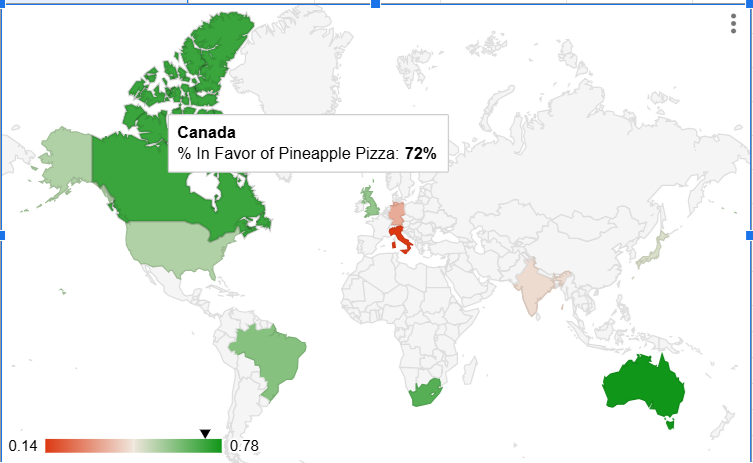
A map chart visualizes data geographically, usually with color gradients, bubbles, or data labels over different regions. As you might imagine, they’re really only useful when location is part of the story. Otherwise, Google Sheets might not generate quite what you had envisioned.
TL;DR: Map charts are great for showing regional differences or concentrations, but can be tricky if your data points are too close together or your audience isn’t familiar with the geography.
Other miscellaneous charts: Best for unique data sets

If your data doesn’t fit any traditional charts and graphs, you can always use one of Google Sheet’s more, eh, unique options.
This includes:
- Waterfall charts
- Histograms
- Radar
- Gauge
- Scorecard
- Candlestick
- Organizational
- Tree map
- Timeline chart
- Table chart
These are typically best used for hyperspecific applications, especially when a typical bar or pie chart can’t accurately represent your data. But please: don’t create an ‘other’ chart just for the sake of making something different (trust us).
How to prepare data for your graph
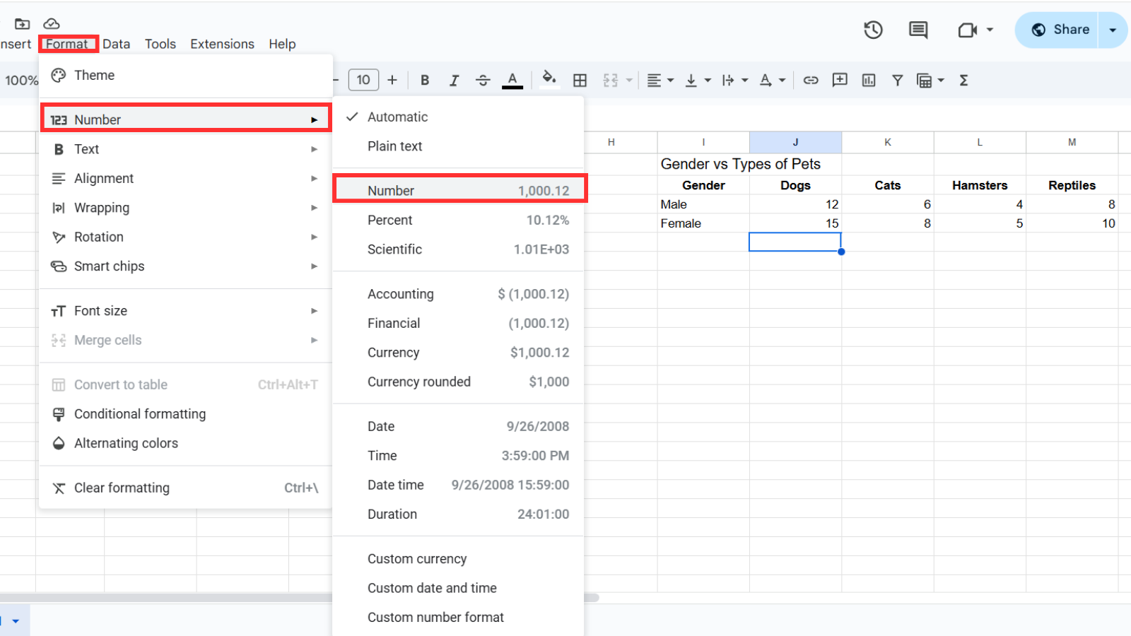
The first step in creating a graph is to prepare your data by formatting it correctly. If the values don’t show up correctly, your spreadsheet might break, which leads to all sorts of problems with visualization down the line.
First, make sure your data is in a table format with headers in the first row. Then, make sure it’s formatted correctly. You can do this by highlighting the data in question, then tapping Format → Number → Number.
Next, be sure to use the drop-down menu to select from different chart types. You might realize it’s better to combo charts instead, like creating a bar graph and scatterplot to point out multiple trends.
Customizing graphs in Google Sheets
Now that we’ve explained how to build a graph in Google Sheets, let’s learn how to customize it by accessing the Customization Tab. This will allow you to add data labels, titles, and axis labels, as well as edit minor features like colors or sizes.
Adding data labels and titles
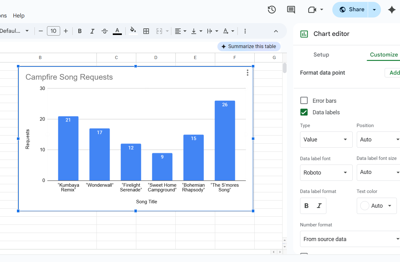
You can add data labels to individual points that provide additional context about your chart (like percentage values in the pie chart). Then, you can add titles to your graph to describe what specific data represents. Google Sheets typically adds these automatically, but you may want to edit them lightly for context.
Here’s how:
- Double-click your chart and open the Customize Tab.
- Under Chart & axis titles, you can add a main title, subtitles, or axis labels.
- For data labels, head to the Series menu and check the box for Data labels. You can even choose placement and formatting options to keep things neat and tidy.
Need to delete items like excess axis labels or data point titles? Just delete them in your data set, or double-tap on your chart to select specific text bubbles.
Adjust the x-axis and y-axis
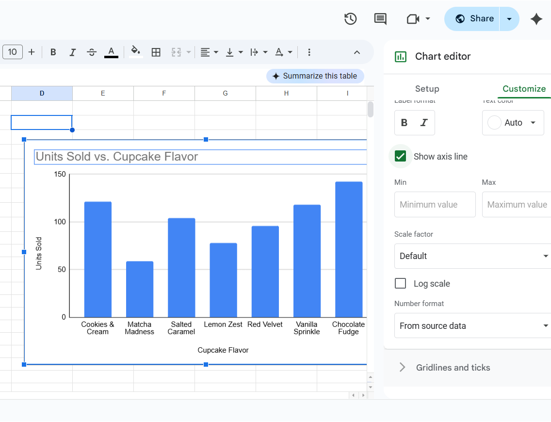
If your chart feels cluttered or a little too empty, it might be time to tweak the axes.
To adjust the x- and y-axis, right-click your chart and hover over Axis. You can choose to edit the Horizontal axis or Vertical axis by adjusting min/max values, changing fonts or spacing, or adding axis titles for extra clarity.
Need to delete extra axis labels? Just uncheck the corresponding boxes in the customization panel. You can also click directly on the item you wish to remove and hit the Delete key.
Chart styles
You’re always welcome to refine your graph by adjusting the data range, chart type, and picking a new chart under Chart type. From here, you can tweak just about everything, from chart style and color schemes to font sizes and background fill.
It’s also where you can change the chart layout to better fit your data — like switching from a line chart to a scatter plot, or experimenting with 2D radar charts (yes, that’s a thing).
Want more clarity? Consider adding a vertical axis title to provide more context.
And remember that you can always experiment with different chart types and customization options to find the best representation of your data.
Add gridlines
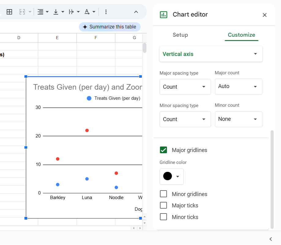
You can also add gridlines to make your graph easier to read. These are particularly useful for showing progression, benchmarks, and other ‘segments’ so your readers can interpret the core values quickly.
Start by right-clicking your graph or double-clicking the area where gridlines are/should be. You should see a menu for Gridlines & ticks. This will allow you to adjust the horizontal and vertical axes, change spacing types, and add or subtract major/minor gridlines/ticks.
For gridlines, you can customize colors. For ticks, you can adjust the length, thickness, and position in the dash.
You can always delete items like gridlines by simply unchecking the tick boxes. For example, you might want to keep minor gridlines and ticks, but remove major gridlines for a better overall look.
Change the legend
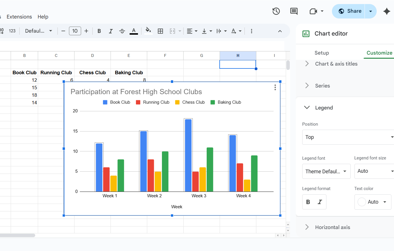
A legend describes the data source you’re using and helps readers understand what each color, line, or bar actually means. This is especially helpful if you’re dealing with multiple data sets or comparisons that might require a little more explanation.
To adjust the legend, double-click your chart or right-click directly on its existing legend. From there, you can click Customize and open the Legend menu. You’ll be able to reposition the legend (top, bottom, right, etc.), change font styles, and pick custom colors that align with your brand or make things easier to read.
Want to hide the legend altogether? Just select None under the position dropdown.
Just keep in mind that avoiding a legend only works for simple graphs. If your chart looks like a rainbow or has lots of complicated details, your audience will thank you for leaving it in.
How to export a Google Sheets graph
Once you have created and customized your graph, you can move it around however you please.
The first option is inserting your graph into another part of your Google Sheets spreadsheet. By this, we mean using the click and drag method to move your graph to a new tab or a new position in your spreadsheet.
Another option is to copy your chart into another Google service — think Docs, Slides, or Vids. To do this, you might tap the chart and copy it (hotkey Ctrl+C), then paste it into documents, slideshows, or video editors (hotkey Ctrl+V). You could also tap File → Download, then create a PDF that can be converted into other file formats.
You’ll also see two built-in methods of exporting your data sandwiched in the three-dot menu at the top right of your chart. See here:
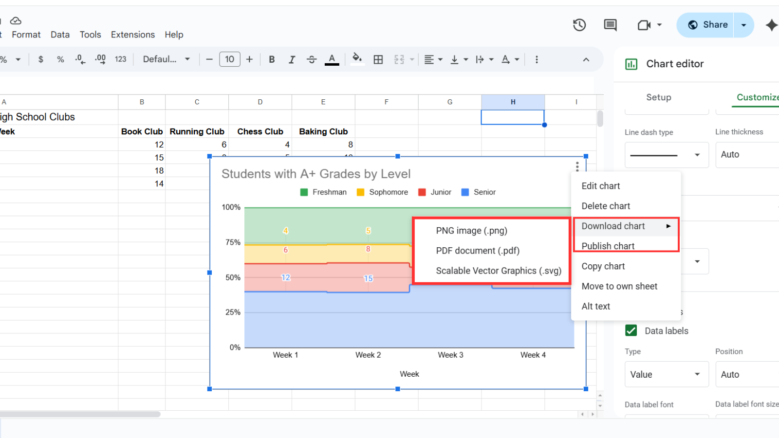
You’ll have two options:
- Download. You can download the chart by itself as a .PNG, .PDF, or .SVG (a scalable vector graphic).
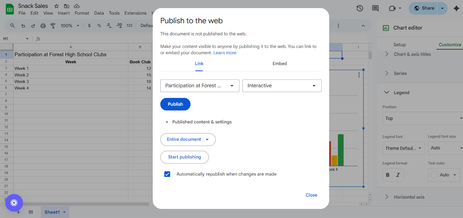
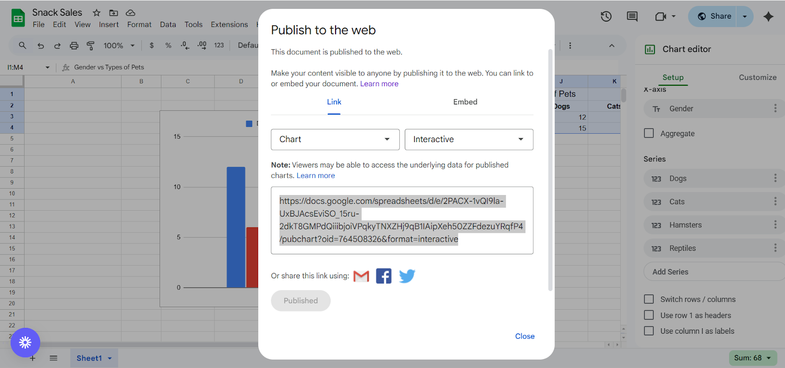
- Publish. You can publish directly to the internet (either as an interactive chart or as an image), then set it to automatically update as changes are made. But you could also opt to embed your graph: Google Sheets lets you copy and paste HTML so you can embed your content directly into a blog or website.
But perhaps the easiest option here is simply to share the spreadsheet with your team. Simply tap Share at the top right, update General access (i.e., add emails or make the link public), then tap Copy link for the updated link. Coworkers will now have the ability to read, comment, or edit depending on their access level. No more stressing about corrupted data now!
Best practices for creating graphs in Google Sheets
As you build data visualizations in Google Sheets, don’t forget to:
- Write a clear and concise title. Do your best not to let it run long, which might get it truncated (aka, shortened) by Google Sheets.
- Make sure your graph is easy to read. If you’re having trouble understanding it, there’s a good chance someone else will, too.
- Consider making different chart types to display your data. That way, you can easily pick and choose between charts. It helps that it only takes a couple of seconds to make each chart.
- Use the chart editor to add and customize data labels and titles. Sure, auto-formatting is pretty cool, but it’s not always correct (or relevant to your data). It’s a good idea to customize your graph a bit more to edit for clarity and make sure it reflects what you’re looking for.
- Be mindful of whitespace and font size. Less is more, as the saying goes. It will also make it easier to move and manipulate your chart.
- Follow proper data visualization techniques. The goal should be to tell a story with your data, and not necessarily throw numbers on the screen. That, of course, is what dedicated data visualization tools are for. 😉
Troubleshooting common chart issues with Google Sheets
Common issues (and solutions!) when creating graphs may include:
Incorrect data ranges or chart types
There are a few different ways to resolve this quickly:
- Double-check the data range. Sometimes, your chart is simply pulling from the wrong cells — like that rogue header row you meant to skip.
- Switch up your chart type. A pie chart can’t display multiple rows the same way a line chart can. If things look wonky, try changing the visualization entirely to see what fits best.
- Reformat as ‘numbers.’ You might have inadvertently changed the format of a few rows of data. And even if they look like numbers, they might be formatted as text in Google Sheets. To fix this, click and drag over the cells that aren’t working. Then, click Format → Number → Automatic. The data should now be ‘valid’ to use in your chart.
Sidenote: if you’re a fast-growing business or an enterprise brand, you might be worried about possible security events. If so, it might be useful to have a tool like Cloudflare, which comes with ray ID so you can check for unauthorized data access.
Google Sheets bar chart not showing
To solve this, you might:
- Reloading the page. You’ve probably already attempted this, but it’s still worth a try.
- Checking your data for errors or inconsistencies. Maybe there’s a wonky formatting issue, or maybe you forgot to enter an extra zero somewhere.
- Checking the formatting. If Google Sheets doesn’t recognize your data as numerical values, it may not display your graph correctly. You can solve this by highlighting the relevant data, then clicking Format → Number → Automatic.
Remember: you can always use the Google Sheets help resources to find solutions to common issues, quickstart guides, troubleshooting forums, and more.
Google Sheets link not opening
If you can’t open a link in Google Sheets to view a chart or graph, you might try:
- Switching Google accounts. You might have access to a link or graph in one account, but not necessarily in another.
- Accessing the link from another device. Some users say the iOS and Android apps can be a bit squirrelly with visualizations.
- Placing the link in another cell. You might be surprised how often this does the trick.
How to get a Google Sheets graph on digital signage
Building your graph was just the first step — and now, you’re looking to put it on the big screen.
Truthfully, we don’t really endorse Google Sheets graphs as the best way to share data. But it’s still totally possible with a free Fugo account.
Here’s the process at a glance:
- Click on File → Share → Publish to the web.
- Copy the link.
- Open Fugo (or sign up for a free 14-day trial).
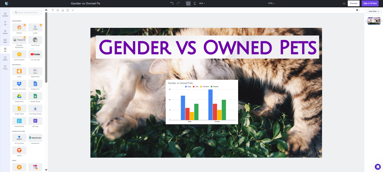
- Head into the Fugo Design Studio. You can customize the titles, backgrounds, and other assets however you please.

- Next, click Apps → Web Page widget. It should look something like this:

- In the top left corner, paste the published link to your Google Sheets graph. Remember that you set it to update automatically, so your digital signage will change as you (or your team) make edits to the spreadsheet.
- Resize and stylize. You can adjust the layout, background, or even stack multiple widgets for a full dashboard-style view.
And voila! You’ve got your live Sheets graph on TV, without copy/pasting or screenshotting your entire computer.
Just keep in mind that Google Sheets graphs are fairly static in terms of design. Fugo’s digital signage content will update with your Sheets, sure, but you won’t be able to customize them as much as data visualization tools like Looker and Tableau.
Which brings us to...
When Sheets graphs aren’t enough
Don’t get us wrong here — Google Sheets is a great place to start with data visualization. But as your business starts growing (and your skills get better), those bare-bones graphs will start showing their cracks.
Think about it:
- You still need to manually format each graph. Not fun, and not quick.
- You’ll have limited sharing and permissions, especially across teams and roles. Security risks, anyone?
- There’s no built-in way to push your data to TV screens without jumping through a few manual hoops.
This is why more and more teams are switching to prompt-based dashboard tools — ya know, the ones where you type what you want, and an AI agent builds the whole thing itself. 😉
They’re easier, cleaner, and way faster when you’re juggling a million other priorities. And yes, it’s all available with Fugo. You can get just a taste of it in our AI Beta Program.
Curious to learn more about our live TV dashboard tools? We’ve got a guide for that, too.
Frequently asked questions about how to make a graph in Google Sheets
Q: How to create a graph in Google Sheets?
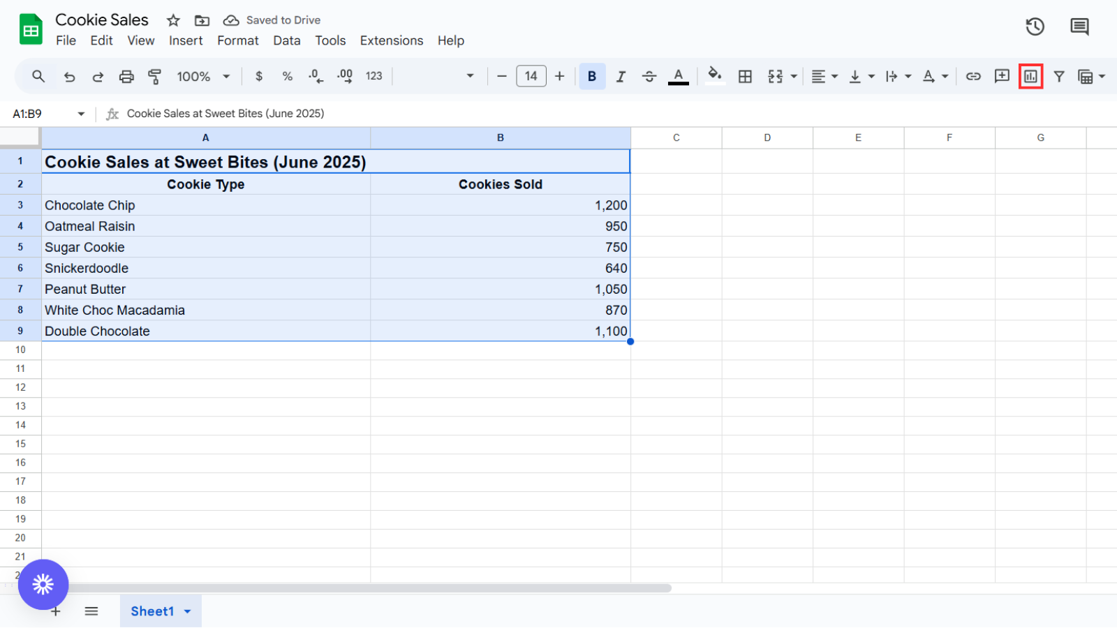
First, enter your data into the spreadsheet. Then, highlight the values you want to turn into a graph. All that’s left is to tap the Chart-shaped button, and Google Sheets will create a graph. You can always update the appearance later in the Customization Tab.
Q: How to make an xy graph in Google Sheets?
Google Sheets refers to XY graphs as ‘scatterplots’ or ‘scatter charts.’ To make one, highlight your data, tap the Chart-shaped button, then select ‘scatter chart’ (if it’s not automatically created for you).
Q: How to automatically make a graph in Google Sheets?
To automatically make a graph in Google Sheets, select your data source and tap the Chart-shaped button on the top right of the interface. Google Sheets will automatically generate a chart style based on what it supposes is the ‘best’ option for your data. However, you can always customize the chart to your liking by accessing the Customization Tab.
Q: How do I make a simple bar graph in Google Sheets?
First, select your data. Then, click Insert → Chart. You can select Bar chart from the drop down menu, then customize the colors, axis titles, and display to your liking.